The outline of Gradient Descent

“A gradient measures how much the output of a function changes if you change the inputs a little bit.” — Lex Fridman (MIT)

Gradient Descent is one of the most known optimization techniques. It is the hot topic for every Machine learner and is also one of the vital the topics.

Optimization is always one of the foremost tasks which tell about the performance of our model. Optimizing is basically bringing out the best possible output. This needs to be done to ensure that the output we are getting is accurate or not. But since, in deep learning, we don’t know that the output we are getting from the new data fed in it or if this is the one we need or not, then what to do?

So, here we use some techniques. One of them is Gradient Descent. Let us discuss it in detail.

What is Gradient Descent?

Let us take an example of mountaineering.

Imagine you are at the top of a mountain, and you have to reach a lake which is at the lowest point of the mountain. Also, you are blindfolded. So, what approach you think would make you reach the lake?

 

A blindfolded person trying to climb mountains, Source: [1]

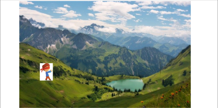
The best way is to observe the ground and find where the land tends to descend. This will give an idea about the direction you should take your first step in.

You may just start climbing the hill by taking really big steps in the steepest direction, which you can do, as long as you are not close to the top. As you come further to the top, you may take smaller and smaller steps, since you may don’t want to overshoot it. This process can be described mathematically, using the gradient.

Have a look at the picture below. Imagine it illustrates our hill from a top-down view, where the red arrows show the steps of our climber. Think of a gradient in this context as a vector that contains the direction of the steepest step the blindfolded man can go and also how long this step should be. To understand it better, look at the graph below:

Top-down view of the hill, Source: [2]

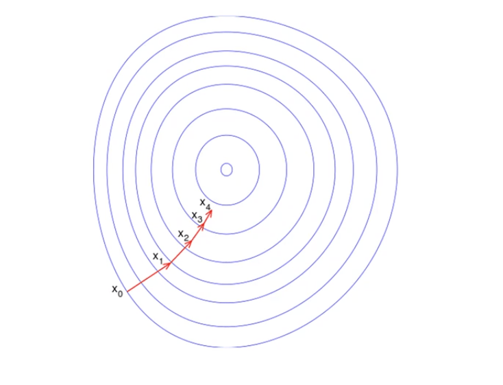
Note that the gradient ranging from X₀ to X₁ is much longer than the one reaching from X₃ to X₄. This is because the slope of the hill is less there, which determines the length of the vector. This is perfectly illustrated in the example of the hill because the more you climb the hill, the less steep it gets. Therefore a reduced gradient goes along with a reduced slope and a reduced step-size for the hill climber.

 

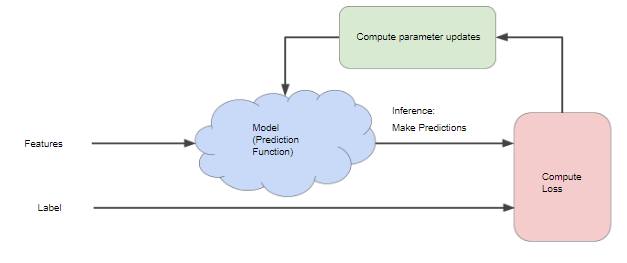
By training the neural networks, we mean that we are calculating the loss function and minimizing it. The value of the loss function tells us how far from perfect the performance of our network on a given dataset is.

Generally, we can define the process of gradient descent as

<span id="MathJax-Element-4-Frame" class="MathJax" data-mathml="θi:=θi+Δθi”>θi:=θi+Δθi

where

<span class="MathJax" data-mathml="Δθi=−α∂J(θ)∂θi”><span class="MathJax" data-mathml="Δθi=−α∂J(θ)∂θi”>Δθi=−α(∂J(θ)/∂θi)<span id="MathJax-Element-6-Frame" class="MathJax" data-mathml="Δθi”>

<span id="MathJax-Element-6-Frame" class="MathJax" data-mathml="Δθi”>Δθi is the “step” we take while walking along the gradient and we set a learning rate <span id="MathJax-Element-7-Frame" class="MathJax" data-mathml="α”>α, to control the size of our steps.<span id="MathJax-Element-6-Frame" class="MathJax" data-mathml="Δθi”>

How it works

Gradient Descent is climbing down the valley rather than moving up i.e. it is a minimization algorithm which minimizes a given function.

b = a – ϒ ∇ f(a)

The equation above describes Gradient Descent’s working.

• “b” describes the next position of our climber,
• “a” represents his current position.
• The minus sign refers to the minimization part of gradient descent.
• The “gamma” in the middle is a waiting factor and
• The gradient term ( Δf(a) ) is simply the direction of the steepest descent.

Importance of the Learning Rate

The steps taken by the Gradient Descent into the direction of the local minimum are determined by the so-called learning rate. It determines how fast we are moving towards the optimal weights.

In order for Gradient Descent to reach the local minimum, we have to set the learning rate to an appropriate value, which is neither too low nor too high.

This is because if the steps it takes are too big, it may not reach the local minimum because it just bounces back and forth between the convex function of gradient descent. Like you can see on the left side of the image below, if you set the learning rate to a very small value, gradient descent will eventually reach the local minimum but it will take too much time like you can see on the right side of the image.

Big and small Learning Rates, Source: [2]

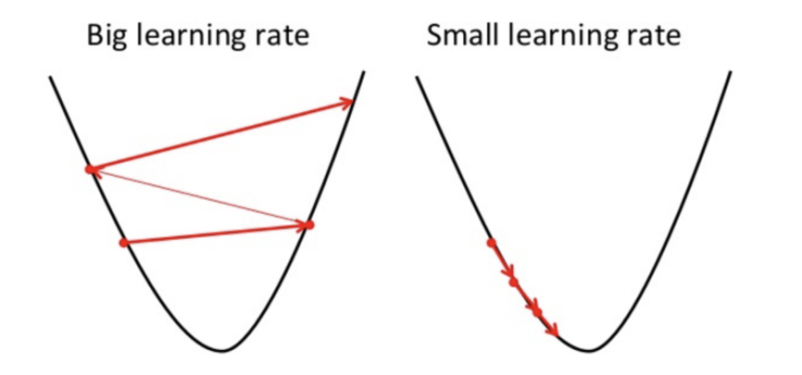
This is the reason why the learning rate should be neither too high nor too low. You can check the learning rate by plotting it on a graph.

The procedure followed, Source: [4]

How to make sure that it works properly?

Let us plot the Cost Function as the Gradient Descent runs. Put the number of iterations on the x-axes and the value of the cost function on the y-axes. This enables you to see the value of cost function after each iteration of gradient descent. This lets you easily spot how appropriate your learning rate is. Just try different values for plotting them all together.

One such instance of a plot is shown below. On the left and the right shows the difference between good and bad learning rates:

Difference between good and bad learning rates, Source: [2]

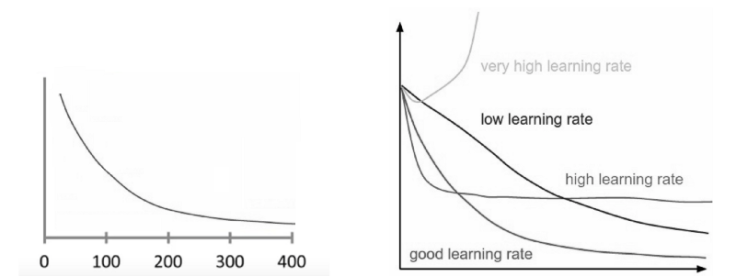
If cost function is decreasing after every iteration, gradient descent is working properly.

When the cost function stops decreasing, it is said to have been converted. Note that the number of iterations needed to converge the Gradient Descent varies. It may take 50 or 60,000 or even millions of iterations to converge. Hence, they are hard to estimate in advance.

Conclusion

In this blog, you got to learn about the basic terms related to Gradient Descent and how the algorithm works at behind. Also, we discovered the concept of Learning Rate and why is it useful.

In the upcoming blog, you will learn about the types of Gradient Descent which will help you train the model more effectively.

References

1. https://leadingindia.ai/
2. https://www.analyticsvidhya.com/blog/2017/03/introduction-to-gradient-descent-algorithm-along-its-variants/
3. https://towardsdatascience.com/gradient-descent-in-a-nutshell-eaf8c18212f0
4. https://www.jeremyjordan.me/gradient-descent/
5. https://medium.com/diogo-menezes-borges/what-is-gradient-descent-235a6c8d26b
6. https://blog.paperspace.com/intro-to-optimization-in-deep-learning-gradient-descent/